In this part of the series, I want to share how I imagine data flowing throughout the BigQuery in the MiWaitWay project.
To learn more about the MiWaitWay project and its high-level architecture, check the introduction article.
You can also find a previous part of the series where I deploy Apache Airflow on a small VM on Google Cloud.
Recap on the project goal
Let me quickly summarize the end goal of the MiWaitWay project. Using GTFS Static and real-time data provided by the MiWay transportation agency, I want to build a dashboard allowing users to select a stop and see the average wait time for different bus lines at that stop. To achieve this, I will need to import and process data in the Google BigQuery, the data warehouse I decided to use.
Data granularity and lifetime
I decided to allow users to see statistics aggregated per day. Calculating the average wait time per hour is not very beneficial, as there are insufficient data points. The average time will be calculated for a complete day only. It will be possible to see the stats for the previous day, the last seven days, or the previous month.
To avoid unnecessary spending, I will limit the lifetime of the real-time data to one month.
Data flow
Below, you can find the data flow diagram I have in mind.
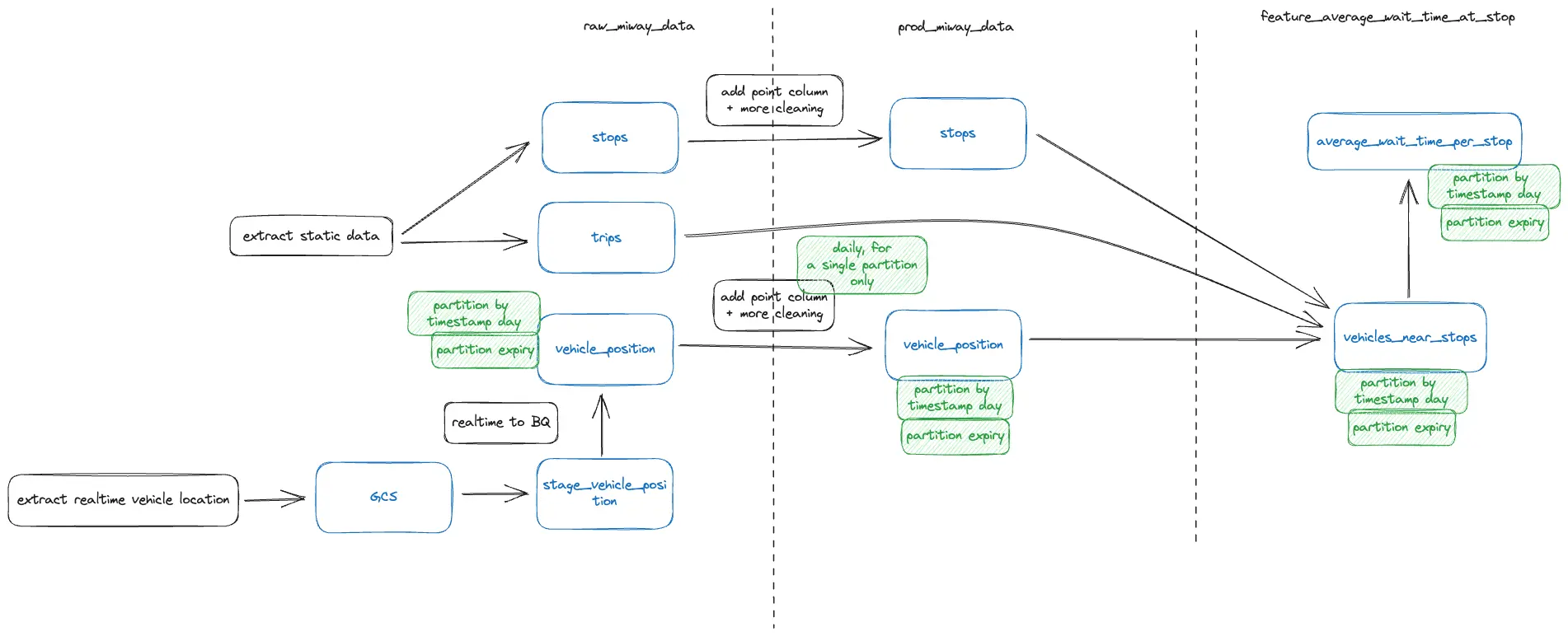
It has three areas:
- raw_miway_data, where raw static (stops, trips, etc.) and real-time (vehicle positions) GTFS data is ingested;
- prod_miway_data, where data from raw_miway_data area is cleaned and enriched;
- feature_average_wait_time_at_stop, where the final results for our particular feature will be stored.
I want to share a few key highlights from the data flow diagram.
The raw static data will be ingested once a day. It doesn’t change often, so running it frequently is unnecessary. I might also consider running the pipeline only once per week.
The extract-realtime-vehicle-location pipeline will continuously save real-time vehicle position batches in files on Google Cloud Storage (GCS). Then, every 30 minutes (can be adjusted), the files will be loaded by the realtime-to-BQ pipeline into BigQuery via a staging table called stage_vehicle_position. This approach will allow BQ queries to be run only once per X minutes instead of every time a small batch of vehicle location data is incoming. I will discuss real-time GTFS later in the series.
The vehicle location tables will be partitioned by the data extracted from the vehicle location’s timestamp. The partitioning allows the efficient running of daily queries. BigQuery documentation on partitioning
The partitions in the vehicle location tables will expire in 30 days. In other words, partitions older than 30 days will be deleted automatically. This reduces the size of the table and avoids unnecessary costs. BigQuery documentation on partition expiry
The pipelines to transform data from raw_miway_data to prod_miway_data will run once a day. They will process data for the previous day. We can use partitions to select the previous day’s data efficiently.
The columns related to the location will be converted to the GEOGRAPHY data type to leverage BigQuery geospatial functions for best performance. The conversion will happen when data is transformed from the raw_miway_data to the prod_miway_data area. BigQuery documentation on working with geospatial data
The last area, feature_average_wait_time_at_stop, will contain the calculated average wait time per stop. The vehicles_near_stops table will contain events when the bus location was registered near the stop. The “average_wait_per_stop” table will contain the final aggregated results that can be used later by the web app and displayed to the user.
Additional changes will likely be required as I work on this project, but I am happy I have a high-level framework written down. In the next article, I will implement static GTFS data ingestion into the raw_miway_data area.
Thank you for reading. Have a great day!